[KM] ♥Keep_Mailing♥ Excel Tip: Searching and Highlighting

Many of us use spreadsheets to manage huge lists of data, like customer data bases, salesperson data bases etc.

Today we will learn a little conditional formatting trick that you can use to search a worksheet full of data and highlight the matching cells.

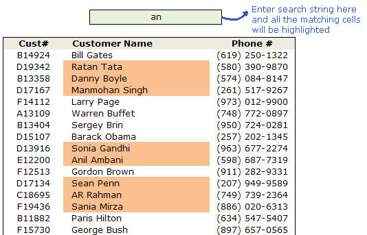
First identify which cell you want to use as search bar. Lets say we choose F4.

Now, Select the data cells you want to search and go to conditional formatting.

We will write a simple formula that returns true if a cell has the content you typed in the search bar (F4) and false if the cell doesnt. You can try something

like

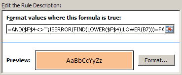
ISERROR(FIND(LOWER($F$4),LOWER(B7)))=FALSE.

But there is a problem with this, it returns true when the search bar is empty, and thus you end up highlighting all cells. So we add a further condition that will highlight the matched cells only if the search bar contains some data.

The formula looks like,

=AND($F$4<>"",ISERROR(FIND(LOWER($F$4),LOWER(B7)))=FALSE)

Finally set the formatting you want to use. I choose dull orange color. You can choose blue, green or pink too.

Hit ok and you are good to go.

M Junaid Tahir www.DailyTenMinutes.com

     

--
You received this message because you are subscribed to the Google Groups "Keep_Mailing" group.
To unsubscribe from this group and stop receiving emails from it, send an email to keep_mailing+unsubscribe@googlegroups.com.
To post to this group, send email to keep_mailing@googlegroups.com.
Visit this group at http://groups.google.com/group/keep_mailing?hl=en-US.
For more options, visit https://groups.google.com/groups/opt_out.