Imagine you have a worksheet with lots of charts. And you want to make it look awesome & clean.
Solution?
Simple, create an interactive chart so that your users can pick one of many charts and see them.
Today let us
understand how to create an interactive chart using Excel.
PS: This is a revised version of almost 5 year old article – Select & show one chart from many.

Feeling excited? read on to learn how to create this.
Solution?
Simple, create an interactive chart so that your users can pick one of many charts and see them.
Today let us
PS: This is a revised version of almost 5 year old article – Select & show one chart from many.
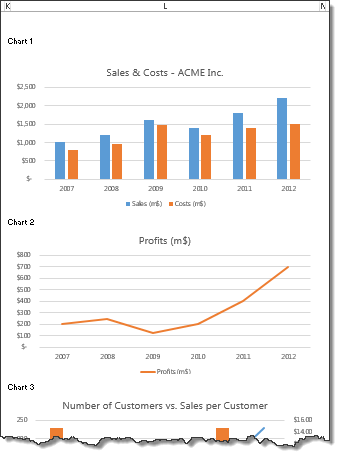
A demo of our interactive Excel chart
First, take a look at the chart that you will be creating.Feeling excited? read on to learn how to create this.
Solution – Creating Interactive chart in Excel
- First create all the charts you want and place them in separate locations in your worksheet. Lets say your charts look like this.
- Now, select all the cells corresponding to first chart, press ALT MMD (Formula ribbon > Define name). Give a name like
Chart1.
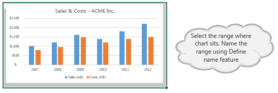
- Repeat this process for all charts you have, naming them like
Chart2,Chart3… - In a separate range of cells, list down all chart names. Give this range a name like
lstChartTypes. - Add a new sheet to your workbook. Call it "Output".
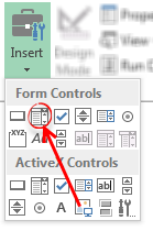
- In the output sheet, insert a combo-box form control (from Developer Ribbon > Insert > Form Controls)
- Select the combo box control and press Ctrl+1 (format control).
- Specify input range as
lstChartTypesand cell link as a blank cell in your output sheet (or data sheet).
[Related: Detailed tutorial on Excel Combo box & other form controls]
- Now, when you make a selection in the combo box, you will know which option is selected in the linked cell.
- Now, we need a mechanism to pull corresponding chart based on user selection. Enter a named range –
selChart. - Press ALT MMD or go to Formula ribbon > Define name. Give the name as
selChartand define it as
=CHOOSE(linked_cell, Chart1, Chart2, Chart3, Chart4)
PS: CHOOSE formula will select one of the Chart ranges based on user's selection (help). - Now, go back to data & charts sheet. Select Chart1 range. Press CTRL+C to copy it.
- Go to Output sheet and paste it as linked picture (Right click > Paste Special > Linked Picture)

- This will insert a linked picture of Chart 1.
[Related: What is a picture link and how to use it?] - Now, click on the picture, go to formula bar, type =selChart and press enter
- Move the image around, position it nicely next to the combo box.
- Congratulations! Your interactive chart is ready

Download Interactive Chart Excel file
Click here to download interactive chart Excel file and play with it. Observe the named ranges (selChart) and set up charts to learn more.You received this message because you are subscribed to the Google Groups "Keep_Mailing" group.
To unsubscribe from this group and stop receiving emails from it, send an email to keep_mailing+unsubscribe@googlegroups.com.
To post to this group, send email to keep_mailing@googlegroups.com.
Visit this group at http://groups.google.com/group/keep_mailing.
To view this discussion on the web visit https://groups.google.com/d/msgid/keep_mailing/CAG%3DbiTsZw4vtvy51h%2BTTsgeYpTksyaX1c3CS_P_u%2BBb5ZfQNFQ%40mail.gmail.com.
For more options, visit https://groups.google.com/d/optout.
No comments:
Post a Comment