[ ::: ♥Keep_Mailing♥ ::: ]™ Excel Tip – Create a Drop Down list with Search Suggestions

We all use Google as a part of our daily routine. One of its feature is search suggestion, where Google acts smart and gives us a list of suggestions while we are typing.

Today in this blog post I will show you how to create this search suggestion in a drop down list in Excel.

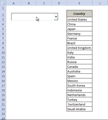
I have a list of Top 20 countries by GDP. I want to create a search suggestion mechanism in a drop-down, which would display the matching options as I type in the search bar. Something as shown below:

To follow along, download the file from here

Here is how you can do this:

1. Insert a Combo Box (ActiveX Control) from the developer tab [Read on how to get the Developer Tab]
2. Right click on the Combo Box and select Properties
3. In the properties dialogue box, make the following changes
   • AutoWordSelect: False
   • LinkedCell: B3
   • ListFillRange: DropDownList
   • MatchEntry: 2 – fmMatchEntryNone

(Note that cell B3 is linked to the Combo Box, which means that anything you type in the Combo Box is entered in B3)

4. Go to Developer tab and click on Design Mode. This will enable you to enter text in the Combo Box
5. Put the following formula in cell F3 and drag it for the entire column (F3:F22)

    =--ISNUMBER(IFERROR(SEARCH($B$3,E3,1),""))

This formula returns 1 when the text in the Combo Box is there in the name of the country on the left. For example, if you type UNI, then only the values for United States and United Kingdom are 1 and all the remaining values are 0

6. Put the following formula in Cell G3 and drag it for the entire column (G3:G22)

    =IF(F3=1,COUNTIF($F$3:F3,1),"") 

This formula returns 1 for the first occurrence where Combo Box text matches the country name, 2 for the second occurrence, 3 for the third and so on. For example, if you type UNI, G3 cell will display 1 as it matches United States, and G9 will display 2 as it matches United Kingdom. Rest of the cells will be blank.

7. Put the following formula in cell H3 and drag it for the entire column (H3:H22)

    =IFERROR(INDEX($E$3:$E$22,MATCH(ROWS($G$3:G3),$G$3:$G$22,0)),"") 

This formula stacks all the matching names together without any blank cells in between them.

8. Now create a Named Range with the following formula

    =$H$3:INDEX($H$3:$H$22,MAX($G$3:$G$22),1)

9. And the final step. Right click on the Worksheet tab and select View Code. In the section on the right, paste the following code

Private Sub ComboBox1_Change() 
ComboBox1.ListFillRange = "DropDownList" 
ComboBox1.DropDown 
End Sub

 

How to create a named range (for Step#6)

1. Go to Fomulas –> Name Manager
2.  In the name manager dialogue box click New.
3. It will open a New Name dialogue box. In the Name Field enter DropDownList
4. In the Refers to Field enter the formula:  =$H$3:INDEX($H$3:$H$22,MAX($G$3:$G$22),1)

Thats it!! You are all set with your own Google type Search bar for a drop down. For better look and feel, Cover the cell B3 with the Combo Box and hide all the columns with formula. You can now wow people with this amazing trick.

To follow along, download the file from here

 

--
You received this message because you are subscribed to the Google Groups "Keep_Mailing" group.
To unsubscribe from this group and stop receiving emails from it, send an email to keep_mailing+unsubscribe@googlegroups.com.
To post to this group, send email to keep_mailing@googlegroups.com.
For more options, visit https://groups.google.com/groups/opt_out.