
Analyst's life is busy. We have to gather data, clean it up, analyze it, dig the stories buried in it, present them, convince our bosses about the truth, gather more evidence, run tests, simulations or scenarios, share more insights, grab a cup of coffee and start all over again with a different problem.
So today let me share with you 25 shortcuts, productivity hacks and tricks to help you be even more awesome.
Write faster formulas
Writing formulas is a big part of analyst life. Use below tricks to reduce the time you spend writing Excel formulas.
 Use F2 key to edit any cell with formulas. This will put the cursor right the end of the formula.
- Exploit intellisense: Whenever you are typing a formula, Excel shows a list of possible functions / names that start with the same few letters you have already typed. Once the list is small enough, you can use arrow keys (up / down) to pick the function or name you want and press TAB to let Excel type the thing for you. This will dramatically speed up your formula writing process.
- Corner click to auto-fill: Once you have a formula, chances are you want to fill down that formula for rest of the table / range. To do this, just select the formula cell, double-click at bottom-right corner of selection. Bingo, Excel will auto-fill the formula all the way down (as long as there are values in adjacent columns).
- CTRL+Enter to type same formula in a bunch of cells: If you want to have same formula applied to a bunch of different cells, just select them all and type the formula. This will place the formula in top-left cell of the selection. Now, instead of pressing enter, press Ctrl+Enter. Excel will place the formula (and adjust any relative references) in all the cells.
- Debug portions of the formula with F9 key: When working with long formulas, often we come across situations when the result doesn't make any sense. You can debug portions of such long formulas using F9 key. Just select the formula portion and press F9 to see the corresponding result.
Related: More formula shortcuts
Pivot table productivity tricks
Pivot tables are a big part of analyst's life. Use below tricks to work faster with Pivot tables.
- Use ALT+N V to insert a pivot table quickly. Or you can use the old school shortcut (from Excel 2003 days) – ALT + D P
- Double click any value to drill down: When looking at pivot tables, if you want to know which records correspond to a particular total, just double click on the number. This will show a new sheet with only data for that number.
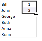
- Rearrange your pivot table items by drag & drop: Want to see a particular product name on top? Want to see the department list in a certain order? No problem. Simple select the items and drag and drop them in any order you want. This will re-arrange the pivot report the way you want.
- Sort quickly with right click: Sort your pivot reports by simply right clicking on the value field and choosing sort option.

Related: Pivot table tricks to make you a star at work
User interaction hacks
A good analyst must create user friendly workbooks because a great deal of the job involves communicating with users. This is where ideas like data validation, form controls & slicers come handy. Here are few hacks to deal with such things faster.
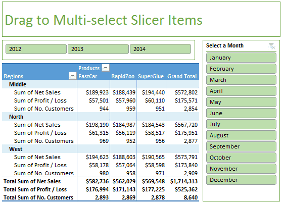
- Multi-select slicer items by dragging: To select multiple items on a slicer, simply drag from first item to last. If the items you want to select are not together, hold down CTRL key and click on one slicer button at a time.
- Set up form control linked cells faster: To set up the linked cell for a form control, simply select the control, click on formula bar, press = and click on the cell you want to link. Done!
- Cut and paste: When setting up a complex workbook model, usually all the calculations are done in a separate worksheet tab. To speed up the process of setting up user interaction elements (such as slicers or form controls), first set them up in the calculation sheet. Once everything is working as per plan, just cut and paste them to the output sheet.
- Alt + Down arrow to pick items from a validation / filter list: Use ALT + down arrow key to pick items from a data validation drop down or filter cells.
- Quickly clear filters with these shortcuts: On a table or list, use CTRL + Shift + L to clear the filters or toggle them. On a slicer use ALT + C to clear the filter (ie select all).
Charting done efficiently
A good chart may get you that hike. So it's no wonder we, analysts spend a lot of time working on charts.
Here are few tricks to work with charts efficiently.
- Use arrow keys to select individual chart elements: When working with charts, we have to select a chart element (bars, columns, titles, axes, legend etc.) before doing anything to it. To quickly select a chart element, simply activate the chart and use arrow keys.

- Adjust chart's source data with drag and drop: If you want to change a chart's source data, simply use drag and drop. Select the chart series (for ex: in a line chart, select the line you want to change). This will highlight the source data range. Now using mouse pointer simply drag and drop the highlighted box to wherever you want. Done!
- Use the select objects tool: When working with multiple charts, often you may want to adjust settings for all in one go. Wouldn't it be great if you can draw a box containing all charts and everything gets selected, a la Power Point (or image editing software)? Well, you can do that in Excel too. Simply activate select objects tool from Home > Find & Select > Select Objects.
In fact, I suggest adding this tool to quick access toolbar (right click on the select objects tool and choose Add to quick access toolbar) so that you can fire it up whenever you want.
- Link chart title etc. to cell value: Default chart titles can be lame and boring. Create awesome titles (subtitles, captions etc. too) by using formulas. Then link them to chart title by using this simple trick. Select the title (or any other element), click on formula bar, press = and click on the cell containing your new title. Bingo, your chart now sports a context-sensitive, smart title. (Related: smart chart titles – how to?)
- Add data to charts with copy paste: Got a chart with sales trend for 3 products and want to add product 4 to it? Simple. Copy the data, select the chart, press CTRL+V. Tell Excel how you want this new data to be pasted and your chart is updated instantly.
Formatting / Presentation tricks
It's no good if you are productive. Your presentation skills are equally (if not more) important.
Let's see some powerful formatting / presentation tricks.
- Format anything with CTRL + 1: Simple, select the cell / chart / image / drawing shape you want to format. Press Ctrl 1. Format as you want.
- Use alignment tools, you must. Hmmm:If your report has multiple charts (or shapes), then align them all, you must. Having perfect alignment doesn't mean you waste several minutes nudging each chart in to right position. Simple select them all (using the select objects tool, of course) and fire up alignment tools from either Page Layout or Format ribbon. Align and space objects in a consistent way.
- Repeat last actions with F4 key: Let's say you are changing font color for various chart elements. You can do this step once on something like vertical axis, then select other items and simply press F4. This will repeat your last action (ie font change) on the new selection.
- Format once, paint many times: Use format painter tool from Home ribbon to quickly apply format settings (including conditional formats) from one range to many. Works awesomely and saves you several precious minutes of formatting time.
- Add frequently used items to quick access toolbar: Formatting tends to be a time consuming activity. To reduce the amount of clicks, mouse travel & un-necessary ribbon navigation, simply add all the frequently used formatting options to quick access toolbar.
- Turn-off grid lines: Get rid of them grid lines to instantly give your workbooks a professional & clean look. You can do this by going to View ribbon. While at it, consider turning-off formula bar & headings too if you find them intrusive
You received this message because you are subscribed to the Google Groups "Keep_Mailing" group.
To unsubscribe from this group and stop receiving emails from it, send an email to keep_mailing+unsubscribe@googlegroups.com.
To post to this group, send email to keep_mailing@googlegroups.com.
Visit this group at https://groups.google.com/group/keep_mailing.
To view this discussion on the web visit https://groups.google.com/d/msgid/keep_mailing/CAG%3DbiTsoxLQ%2BBX72Qth48b%2BgeJyB1ExwYHQ3x%2BFw1gY37YvKiQ%40mail.gmail.com.
For more options, visit https://groups.google.com/d/optout.
No comments:
Post a Comment